 =0.5 as
expected for first-order Fermi acceleration (Bell 1978) and observed in
at least some hotspots (Meisenheimer et al. 1989).
=0.5 as
expected for first-order Fermi acceleration (Bell 1978) and observed in
at least some hotspots (Meisenheimer et al. 1989).
As noted by GCL, the spectral index asymmetry can be explained as a
dilution effect. The hotspot on the jet side is brighter (Bridle &
Perley 1984; Laing 1989) and flattens the overall spectrum more than
the fainter hotspot on the counterjet side. The asymmetry in spectral
index arises if the hotspot spectral indices are reasonably flat,
perhaps with =0.5 as
expected for first-order Fermi acceleration (Bell 1978) and observed in
at least some hotspots (Meisenheimer et al. 1989).
The natural explanation for the enhanced hotspot brightness on the jet
side is Doppler boosting. If the hotspots are moving at velocities  c away
from the nucleus of the radio source at an angle arccos
c away
from the nucleus of the radio source at an angle arccos =
= /2-
/2- to our line of sight then the observed
flux density is (Ryle & Longair 1967; Peacock 1987)
to our line of sight then the observed
flux density is (Ryle & Longair 1967; Peacock 1987)
S = S_0 (1-)^{-(3+)},
(18)
where is the radio
spectral index and I have included the angle independent Lorentz
factors in S_0. Wilson & Scheuer (1983) showed that this
simplified description is valid in practice. For the jets the exponent
is (2+), but I here
consider the hotspots as monolithic entities. The hotspot on the
counterjet side has its flux density correspondingly reduced. The
median ratio of peak intensities is reported by GCL to be 1.37; the
median flux density ratio of 1.24 is smaller because the lobe emission
is unaffected by orientation and dilutes the difference in the
hotspots.
The jet is only a crude orientation indicator, simply indicating which side is which. The asymmetry in hotspot luminosity and spectral index is expected to be small for sources nearly in the plane of the sky, and large for sources close to the line of sight. Similar depolarization behaviour is expected, as sources close to the plane of the sky have similar depolarization on both sides, whereas sources close to the line of sight show a large depolarization asymmetry. In Fig. 4 I show the spectral index difference (counterjet spectral index less jet spectral index) plotted against the depolarization ratio (counterjet side depolarization divided by jet side depolarization) for the GCL and Liu & Pooley (1991) samples.
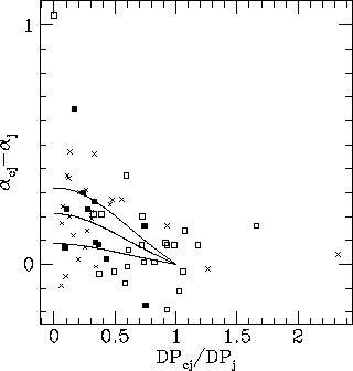
Fig 4. Spectral index difference plotted against depolarization
ratio for the sources in the GCL sample (crosses) and the Liu &
Pooley (1991) sample (filled squares). Lines represent an expected
relation for =0.1, 0.25, and
0.4 (from bottom).
Using both Spearman's rank and Kendall's  , the spectral
index difference and depolarization ratio are anticorrelated at the 99%
confidence level. This is exactly as expected---large differences in
spectral index should be associated with small depolarization ratios.
Furthermore, the zero point of the correlation is correct. As can be
seen in Fig. 4, those sources not at small angles to the line of sight
for which the depolarization ratio is near unity have spectral index
differences which scatter around zero. The amplitude of the scatter is
consistent with measurement errors in the spectral index of about 0.1
(GCL).
, the spectral
index difference and depolarization ratio are anticorrelated at the 99%
confidence level. This is exactly as expected---large differences in
spectral index should be associated with small depolarization ratios.
Furthermore, the zero point of the correlation is correct. As can be
seen in Fig. 4, those sources not at small angles to the line of sight
for which the depolarization ratio is near unity have spectral index
differences which scatter around zero. The amplitude of the scatter is
consistent with measurement errors in the spectral index of about 0.1
(GCL).
I have modelled the spectral index asymmetry as follows. The flux density on the jet side is
S_j = ( /_0)^{-_l}
+ f(_0) (/_0)^{-_h}
g(,), (19)
/_0)^{-_l}
+ f(_0) (/_0)^{-_h}
g(,), (19)
where f is the intrinsic flux density ratio of the hotspot to
the lobe, _l and _h
are the spectral indices of the lobe and hotspots respectively, and
g(,) is the Doppler
beaming factor (equation 18). The total spectral asymmetry can then be
calculated as a function of orientation angle. I take _h=0.6, _l=1.1 and
f=0.5 at 20 cm which can easily give the total flux asymmetry
for =0.2 and
maximises the spectral index asymmetry because for this choice the lobe
and hotspot have comparable fluxes over the range of interest.
A simple model connecting depolarization ratio and angle is needed. At
long wavelengths p  1 / (
1 / (
 ^2), and when
both sides are depolarized the depolarization ratio is simply _+/_-
which depends only on the geometry. I again take m=1, and in
Fig. 4 show the expected relation between the two asymmetries in this
model for =0.1, 0.25 and
0.4. The lines shown are not wholly unrealistic because the two
endpoints are correct and the intermediate variation must be monotonic.
Note that the curves cover the region occupied by the data, and that
the scatter in the spectral index difference increases at small
depolarization ratios consistent with a range of hotspot advance speeds
(or of other source properties).
^2), and when
both sides are depolarized the depolarization ratio is simply _+/_-
which depends only on the geometry. I again take m=1, and in
Fig. 4 show the expected relation between the two asymmetries in this
model for =0.1, 0.25 and
0.4. The lines shown are not wholly unrealistic because the two
endpoints are correct and the intermediate variation must be monotonic.
Note that the curves cover the region occupied by the data, and that
the scatter in the spectral index difference increases at small
depolarization ratios consistent with a range of hotspot advance speeds
(or of other source properties).
The model chosen clearly doesn't give the correct absolute spectral
indices, but these can be obtained simply by adjusting both _l
and _h together.
Doing so has little effect on the asymmetry obtained. Changing the
difference between _l and _h
changes the resulting asymmetry, roughly in proportion. For these
models, with a median angle of 50 degrees to the plane of the sky which
is consistent with the source orientations derived earlier, the median
spectral index asymmetry _cj-_j
 (_l-_h), although
the asymmetry will be reduced for less optimal values of f.
The major result is that reasonable choices of parameters can reproduce
the observed asymmetry.
(_l-_h), although
the asymmetry will be reduced for less optimal values of f.
The major result is that reasonable choices of parameters can reproduce
the observed asymmetry.
Liu & Pooley (1991) also considered Doppler effects. Their reasoning is incorrect as they neglect Doppler boosting entirely, and rely on red- and blue-shifting different portions of a curved spectrum to the observed wavelengths. As the spectral curvature is usually small, the required velocities are large.