Realistic diffusion models

These realistic models cover the full range of electron histories. The JP and KP models are included as special cases. The JP model (with D=0) is a model where the mean free path goes to zero. The KP model is a uniform field with an infinite mean free path. Also presented in Paper I was a model with no scattering in which the electron pitch angle evolved to keep the magnetic flux linked by the electron orbit constant as the field changed, which is a variable field model with an infinite mean free path.

I assume that the scattering mean free path is much shorter than the scale on which the magnetic field varies. This simplifies the problem somewhat, as the electron's pitch angle can be assumed to remain constant between scattering events. This means that if the particle's pitch angle is and it travels a distance s between one scattering event and the next, it travels a distance

= s cos (3)

along a field line, where s is distributed as

p(s) ds = (1/) exp(-s/) ds, (4)

where is the mean free path. I assume that the scattering leads to a new random value of the pitch angle. The position as a function of time is binned to give an energy loss kernel which is the fraction of the electrons lifetime spent at a particular location weighted by sin^2 which is proportional to the losses.

In the models shown in this paper, the electrons have a total path length of 10^4 units and a mean free path of 1, 0.1, and 0.01 units (made up of 10^4, 10^5, and 10^6 steps respectively). There are 4 units per grid cell. On average, the step length parallel to the field is half the total distance travelled, so the rms particle displacement is 12.5, 4.17, and 1.25 grid cells respectively.

A magnetic field model is constructed by choosing Fourier components from a power spectrum (see Tribble 1991). The scale length of the field is set to be 4 grid cells. The three models with three different mean free paths therefore allow the electrons to sample regions somewhat larger, about the same size as, and somewhat smaller than the field's scale size. Models where the rms particle displacement is very much smaller than the scale size of the field, in which electrons only sample the local field should be very close to the simple models considered in Paper I and elsewhere in this paper. The models where the electrons sample a wider range of conditions might be different, because there are still correlations in field strength persisting to large distances and so the region sampled by an individual electron is not representative of the entire volume. This will give a larger scatter in electron losses than the simple models, and the spectrum will also depend to some extent on the detailed form of the magnetic field's power spectrum.

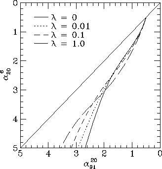
Figure 9. Colour-colour diagrams for the models including inverse Compton losses with B_IC = 0.25B_rms and realistic diffusion in a three dimensional random magnetic field, for the set of frequencies (6, 20, 91) cm.

Starting from a set of initial positions chosen at random, field lines are integrated to give magnetic field strength as a function of path length. The losses for an electron at a given position can be found by convolving a loss kernel with the loss factor B^2 along the field line. A large sample of electron losses is constructed by convolving many kernels with many field lines in many positions. For each realization, this gives the magnetic field in which the electron is currently radiating and the effective field that has determined the energy losses.

Given the current field strength and the losses, this defines a break frequency ' which is

' B/(B_IC^2 + <B^2 sin^2>)^2. (5)

For each electron in the sample, I calculate '. The emission from each electron has an intensity normalization proportional to B^(1+). The density of magnetic field lines is proportional to the field strength, so that to get a uniform electron density we must weight each electron by an extra factor 1/B. I combine all the electrons, weighted by a total factor of B^, to get the distribution of ' which gives the fraction of the emission with a given break frequency.

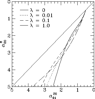
Figure 10. Colour-colour diagrams for the models including inverse Compton losses with B_IC = 0.25B_rms and realistic diffusion in a two dimensional random magnetic field, for the set of frequencies (6, 20, 91) cm.

The total spectrum is calculated by superposing the spectra with different break frequencies and averaging over the emitted angles. The accuracy attainable for these spectra is limited primarily by the sampling of the magnetic field, the number of particles one considers, and the number of bins used in the distribution of '. Unfortunately, the case with no diffusion, which can also be integrated directly, is the most difficult to calculate in this way as there is a long tail in the ' distribution.

I show, in Fig. 9, colour-colour plots for random field models with realistic diffusion, for the case B_IC = 0.25B_rms. Fig. 10 shows colour-colour plots for a two-dimensional random field. Again, as noted earlier, the two-dimensional locus lies slightly closer to the diagonal. The realistic diffusion models give colour-colour loci that are similar to the other models shown in this paper.

On to:

• Two component models

• Index