 _1' contributing a fraction
f_1 of the low frequency flux, and a second component with a
break frequency _2'
contributing the remainder of the low frequency emission (I assume that
_1' < _2').
_1' contributing a fraction
f_1 of the low frequency flux, and a second component with a
break frequency _2'
contributing the remainder of the low frequency emission (I assume that
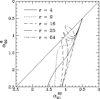
_1' < _2').If the break frequencies of the two components are reasonably well separated, then the spectrum steepens as one component fades, then flattens again until the second component starts to fade. This causes the locus followed in the colour-colour diagram to come back up to the diagonal line, in some cases looping back on itself. Some examples of two component colour-colour diagrams are shown in Fig. 11.
Figure 11. Colour-colour diagrams for the two component models for the set of frequencies (6, 20, 91) cm. 75% of the low frequency flux comes from the component with the lower break frequency, and a variety of models with different ratios r of the two break frequencies are shown.
The two adjustable parameters of the models are the ratio r =
_2'/_1' of the break frequencies, and the
fractional contribution f_1 of the component with the lowest
break frequency component to the low frequency emission. Fig. 11 shows
how the colour-colour diagram depends on the ratio r for a
fixed value of f_1=0.75.
On to:
Up to: ___________________________________ Peter Tribble, peter.tribble@gmail.com